
On this page
Expected shortfall (ES) is the average loss in the worst specified fraction of a modeled loss distribution. At 95% confidence, that fraction is the worst 5%. Unlike a single loss quantile, it uses the severity of the tail.
The confidence level, horizon, loss sign convention and scenario weights must be stated. For discrete outcomes, the tail can include only part of the probability mass at the cutoff. That matters for prediction-market shares, where losses often have a small number of possible values.
Expected shortfall vs value at risk
The Basel market-risk terminology distinguishes VaR, a confidence-level loss threshold over a horizon, from ES, a tail-loss average. Its brief wording is useful orientation; the discrete examples below use an explicit quantile-tail convention.
| Measure | Question answered | What it does not establish |
|---|---|---|
| Value at risk | Where is the chosen loss quantile? | A worst possible loss or the size of every tail loss |
| Expected shortfall | What is the average loss across the worst tail probability? | A maximum loss, correct scenario probabilities or guaranteed capital sufficiency |
| Risk of ruin | Does a process reach a stated failure boundary? | The same quantity as a terminal tail-loss average |
The boundary question is covered separately in our risk of ruin guide. An ES value of 60 does not mean a 60% probability of failure or a maximum possible loss of 60.
State the loss and confidence conventions
Use a random loss L: positive values are losses and negative values are gains. Let alpha be a confidence between zero and one. This page defines VaR(alpha) as the smallest loss value whose cumulative probability is at least alpha.
Expected shortfall then averages the worst 1 −alpha probability mass. In quantile notation:
ES(alpha) =[integral from alpha to 1 of VaR(u) du] /(1 −alpha)
Some references use a tail probability rather than confidence as their level parameter. A level labeled “5%” in one convention can correspond to “95%” in another. Match the convention before comparing results.
Original expected shortfall calculation with a fractional tail
Construct ten equally weighted, one-period loss scenarios in the same fictional currency units:
0, 0, 0, 0, 0, 0, 10, 20, 40, 100
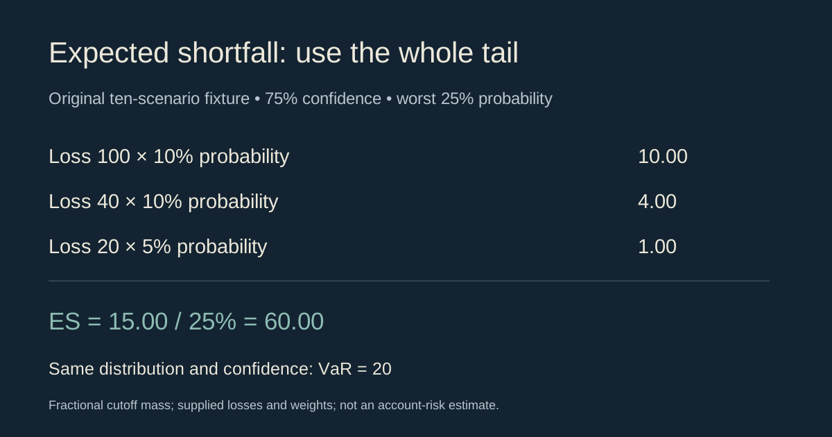
Each scenario has probability 10%. Set confidence to 75%, so the required tail is 25% of probability mass, equivalent to 2.5 equally weighted observations. The deliberately small sample makes the cutoff visible; it is not a recommended dataset for real-world risk estimation.
| Loss, from worst downward | Available probability | Probability used in worst 25% | Loss contribution |
|---|---|---|---|
| 100 | 10% | 10% | 10.00 |
| 40 | 10% | 10% | 4.00 |
| 20 | 10% | 5% | 1.00 |
| Other scenarios | 70% | 0% | 0.00 |
The loss-weighted tail contribution is 15.00. Divide by the tail probability, not by the whole sample:
ES(75%) =(100 ×0.10 +40 ×0.10 +20 ×0.05) /0.25 =60.00
Under the stated empirical quantile convention, VaR(75%) is the eighth sorted observation, 20. Thus this constructed distribution has VaR 20 and ES 60 at the same confidence and horizon.
Why averaging only losses strictly above VaR can be wrong
In that same fixture, the losses strictly above 20 are 40 and 100. Their average is 70, but together they cover only 20% probability, not the required 25% tail. Including every observation at or above 20 instead averages three observations and gives approximately 53.3333, covering 30% probability.
Neither shortcut matches the defined 25% tail. Include exactly the needed half of the cutoff observation’s probability mass. If several tied observations share the cutoff value, their combined contribution can be allocated fractionally without changing the loss value being averaged.
Acerbi and Tasche’s research on expected shortfall explains why definitions that agree for continuous distributions can diverge at discontinuities. This page’s examples use a full fixed-probability tail rather than treating an unqualified conditional average as universally equivalent.
Calculate this expected shortfall example in Excel
Enter the ten supplied losses into cells H2:H11 in descending order: 100, 40, 20, 10, followed by six zeros. For this exact equal-weight 75%-confidence fixture:
=(H2+H3+0.5*H4)/2.5
The result is 60. The first two observations count fully and the third counts half. This formula is intentionally specific to ten equal weights and a 25% tail. It is not a general formula for other sample sizes, confidence levels or unequal scenario probabilities.
Do not replace it with an average of values greater than a spreadsheet percentile. Percentile interpolation conventions and treatment of the cutoff can differ from the explicitly stated empirical-quantile convention here.
Changing confidence changes the tail being averaged
Keep exactly the same ten losses. At 80% confidence, the worst 20% contains losses 100 and 40, giving ES 70 and VaR 20. At 90% confidence, the worst 10% contains only loss 100, giving ES 100 and VaR 40.
| Confidence | Tail probability | VaR | ES |
|---|---|---|---|
| 75% | 25% | 20 | 60 |
| 80% | 20% | 20 | 70 |
| 90% | 10% | 40 | 100 |
These changes follow from the supplied distribution, not a change in its observed data. Comparing two ES values without matching their confidence, horizon, currency and estimation method can be misleading.
A discrete prediction-market example
Construct a separate fictional holding of 100 outcome shares bought for 0.70 each, with a 1.00 ordinary winning payout per share. Exclude fees and every other cash flow. Supply a success probability of 96%; this is an assumption, not an observed platform probability or validated forecast.
Success pays 100 against cost 70, producing profit 30 and therefore loss −30. Failure pays zero, producing loss 70. The modeled loss distribution is 96% at −30 and 4% at 70.
At 95% confidence, VaR is −30 because cumulative probability has already reached 96% at that value. The worst 5% contains all 4% of the 70 loss plus 1% of the −30 gain:
ES(95%) =(0.04 ×70 +0.01 ×(−30)) /0.05 =50
The modeled ES is 50, not the conditional average of 70 obtained by including only losses strictly greater than VaR. A negative VaR also does not mean loss is impossible: the supplied distribution still includes a 70 loss.
Keep real contract rules and costs attached to their instruments. This fictional payout model is not a claim that every Kalshi, Polymarket or other venue outcome always settles under those assumptions.
The same VaR can hide different tail severity
In two more original distributions, let loss be zero with probability 96%. In distribution A, the remaining 4% loses 100; in B, the remaining 4% loses 500. At 95% confidence, both have VaR zero.
But their ES values are (0.04 ×100 +0.01 ×0) /0.05 =80 and (0.04 ×500 +0.01 ×0) /0.05 =400. A quantile that stays unchanged does not imply unchanged tail severity.
Reproduce the calculation in Python
Download the original offline expected-shortfall example. Run python3 expected-shortfall.py. It uses Python’s standard-library fractions for exact weights, checks that probabilities sum to one, and applies partial probability mass at the tail cutoff.
The script verifies the examples against a separate piecewise-linear minimization calculation and checks translation, scaling and invalid weights. It fetches no prices, reads no account data and submits no orders. Its outputs verify arithmetic for the supplied distributions.
What expected shortfall cannot prove
A tail average is conditional on a distribution and method. Missing stressed states, unrealistic probabilities, mismatched horizons and omitted costs can make a precise-looking result uninformative. Repeated observations of one underlying event do not automatically supply independent evidence about rare outcomes.
Backtesting is a separate task: define the forecast timestamp, realized loss, sample selection and statistical procedure before claiming validation. A few quiet periods with no large loss do not independently establish that the tail model is accurate.
ES also does not measure every path event. A position might breach a collateral requirement before its terminal payout. Our liquidation guide and fixed-unit ruin calculator address different questions with their own assumptions.
For reproducible prediction-market research, store the event, outcome, units, costs, horizon, scenario weights, confidence level, quantile convention and tail allocation. Alphascope’s market-linked research adds event context; it does not turn supplied scenario weights into validated probabilities.