
On this page
Risk of ruin is the probability that a process reaches a defined failure boundary under stated rules. A useful answer must specify the starting capital, gains and losses, time horizon, dependence and stopping conditions. A win rate alone does not identify it.
In this guide, “ruin” first means reaching zero in a deliberately simple fixed-unit model. We then explain why that model is not a ready-made estimate of failure for a prediction-market account. The examples are original constructed calculations, not account forecasts.
For the average severity of a modeled loss tail, read our expected shortfall guide. That terminal-loss question is separate from reaching a boundary during a path.
Try the risk of ruin calculator
Our interactive risk of ruin calculator separates zero-before-target probability by a chosen round limit from eventual zero-before-target probability. It also shows paths that have not reached either stopping boundary.
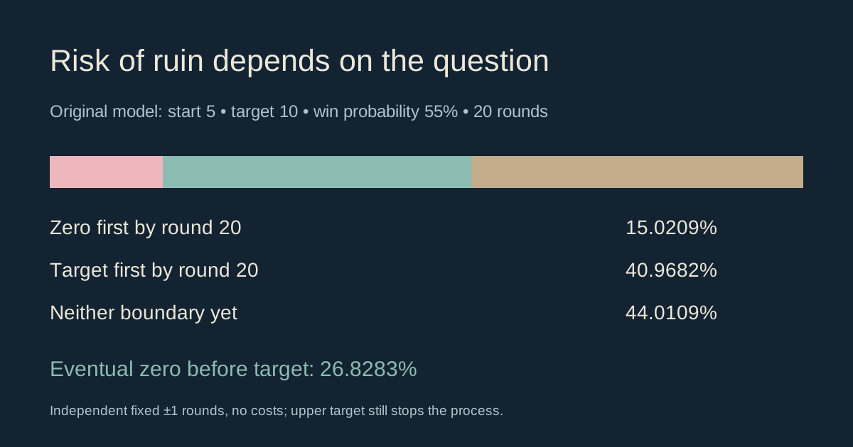
The default example starts at 5 units, stops at 0 or 10, gains or loses exactly 1 per independent round, and uses a constant 55% win probability. Those are supplied assumptions, not a measured trading edge.
Define ruin before calculating it
Reaching zero, losing half the starting capital, breaching a maintenance requirement and running out of available cash are different events. A calculation for one boundary cannot silently stand in for the others.
| Question | Definition needed |
|---|---|
| Can capital hit zero? | Absolute lower capital boundary |
| Can losses reach a threshold? | Threshold relative to starting capital or a running peak |
| Can an account be liquidated? | Venue-specific collateral and maintenance rules |
| Can money become unavailable? | Cash, collateral, settlement and withdrawal timing |
A drawdown from a running peak is path-dependent: the reference peak changes. The calculator on this page uses fixed absolute boundaries instead. It does not estimate a moving drawdown or an exchange liquidation probability.
The classical fixed-unit model
MIT’s stochastic-processes lecture presents independent fair rounds with a one-unit gain or loss and stopping at zero or an upper target. In that fair model, the chance of reaching the upper target first is starting units divided by target units.
For our generalized teaching model, let k be starting units, N the upper target, p the probability of gaining one unit, and q =1 −p the probability of losing one. Every round is independent, p remains constant, and reaching either boundary ends the process permanently. There are no costs, deposits or changes in unit size.
Risk of ruin formula with two boundaries
Write R(k) for the probability of reaching zero before N. Condition on the next round:
R(k) =p ×R(k +1) +q ×R(k −1), with R(0) =1 and R(N) =0.
This recurrence expresses the complete model: from k, the next state is k +1 or k −1. Solving its boundary conditions gives, for p neither zero, one nor one-half:
r =q /pR(k) =(r^k −r^N) /(1 −r^N)
For p =0.5, the result is R(k) =1 −k/N. At p =0, the process loses every round and eventually reaches zero; at p =1, it reaches the upper target without ruin. These statements apply only to the stated process.
“Eventually” removes the round limit but keeps the upper stopping boundary. It does not mean trading forever after reaching the target. Dropping that stop defines a different problem and can produce a different probability.
An original example with only four two-round sequences
Start with 1 unit, stop at 0 or 3, use fair independent rounds and a horizon of 2 rounds. Each two-round win/loss sequence has probability one-quarter. Once a boundary is reached, subsequent hypothetical coin results no longer change the stopped state.
| Supplied sequence | Stopped-state path | State by round 2 |
|---|---|---|
| Loss, loss | 1 →0 →0 | Ruined |
| Loss, win | 1 →0 →0 | Ruined |
| Win, loss | 1 →2 →1 | Neither boundary |
| Win, win | 1 →2 →3 | Upper target |
By round 2, ruin probability is 50%, target probability is 25%, and unresolved probability is 25%. The three sum to 100%. The eventual formula gives 1 −1/3 =2/3, or approximately 66.6667% ruin before the target.
The unresolved quarter cannot be labeled a success just because it has not failed yet. It also cannot all be labeled a future failure. Continuing those paths under the model supplies the missing distinction.
Finite-horizon risk is different from eventual risk
For the calculator’s separate default model, k =5, N =10, p =0.55 and a 20-round horizon. Forward propagation gives approximately:
- Reached zero first by round 20: 15.0209%.
- Reached the upper target first by round 20: 40.9682%.
- Neither boundary reached by round 20: 44.0109%.
The eventual zero-before-target probability is approximately 26.8283%. The difference comes from allowing unresolved paths to continue. It is not a new probability estimate inferred from market prices.
At a zero-round horizon, neither boundary has been reached from an interior starting state, so the finite-horizon ruin and target probabilities are both zero. The eventual result remains unchanged because its question has no round limit.
Why prediction-market win rates are not enough
Consider an original outcome-share example: buying one share at 0.80 that pays 1.00 if the event occurs produces a 0.20 gain on success versus a 0.80 loss on failure, before costs. The payoff is asymmetric, unlike the calculator’s equal one-unit gains and losses.
Suppose, solely for arithmetic, the event’s true success probability were 75%. Expected profit would be 0.75 ×0.20 +0.25 ×(−0.80) =−0.05. A high supplied win probability can coexist with negative expected profit. It is not interchangeable with the p input of a symmetric one-unit process.
Realized win rate, forecast accuracy and economic edge also differ. A small, selected record of winning trades does not validate a stable probability or independence assumption. Use the expected-value calculator to keep probability, cost and payout separate.
Correlated outcomes can invalidate independent-round assumptions
Several positions may depend on the same event, data release or underlying driver. Counting them as separate independent trials can misrepresent the distribution of combined losses.
As a constructed comparison, two identical exposures to one event paying zero with probability 30% fail together with probability 30%. If two failure events were genuinely independent and each had probability 30%, both failing would have probability 9%. Similar marginal probabilities do not identify their dependence.
The joint-probability calculator illustrates that distinction. It does not determine the actual dependence between market contracts. Read exact event definitions before treating prices as observations of separate risks.
What this calculation leaves out
Fees, spread, changing order size, partial fills, borrowing costs, leverage, transfers and delayed settlement all change the cash process. A sequence of net profits and losses with unequal magnitudes requires a richer model than the fixed-unit formula.
Model uncertainty matters too: knowing a formula exactly does not mean its p input is known. Scenario analysis can show how a supplied assumption changes an output; it does not turn that assumption into verified evidence.
For a venue-specific maintenance event, read our liquidation explanation. Liquidation is not necessarily zero account equity, and a general gambler’s-ruin calculation does not replace the venue’s risk rules.
Make the research reproducible
- Define the exact lower boundary and upper stop, if any.
- State the horizon and whether crossing is measured during the path.
- Specify every possible gain, loss and cost.
- Separate supplied probabilities from estimates and observed records.
- Document dependence, changing stakes and account cash flows.
- Keep unresolved paths in the reported distribution.
- Use a model matched to the actual question before interpreting the number.
The calculator uses direct state propagation for finite horizons and a stable evaluation of the two-boundary formula for eventual risk. We checked short paths by exhaustive enumeration and the eventual results against the backward boundary equations. These checks validate the implemented teaching model, not any trader’s real-world failure probability.
Alphascope’s market-linked research helps investigate event context. It does not establish a forecasting edge or supply a personal ruin-probability estimate.