
On this page
Platt scaling fits a sigmoid mapping from model scores to probabilities. Isotonic calibration fits a more flexible, non-decreasing mapping. Both need data for fitting and a separate evaluation to determine whether the mapping helped. A smaller calibration error on the fitting sample is not sufficient evidence.
This guide is for people evaluating binary forecasts, including prediction-market research. It does not calibrate a live Kalshi or Polymarket account. Its downloadable example uses generated classification data, not market outcomes or Alphascope forecasts.
What is Platt scaling?
The scikit-learn calibration guide gives the sigmoid form p = 1 / (1 + exp(Af + B)), where f is a classifier score and A and B are fitted parameters. Some explanations use sigmoid(af + b), which reverses the parameter signs. Check the convention before copying coefficients.
A classifier score is not automatically a probability. Likewise, a market price, a language model’s verbal confidence, and a stored model margin are different inputs. Decide what your mapping receives and document it. For a Yes/No forecast, also define which outcome is the positive class.
Imagine a fictional mapping p = sigmoid(0.5f). At scores −2, 0 and 2 it returns about 26.894%, 50% and 73.106%. These numbers illustrate the shape; the coefficient was chosen by hand. They are not fitted parameters, a validation result, or a suggestion to halve your own model’s scores.
What is isotonic calibration?
Isotonic calibration allows a non-decreasing mapping rather than restricting it to a sigmoid. It can introduce flat regions and tied probabilities. That flexibility also creates more opportunity to overfit a small calibration sample. The official guide discusses these tradeoffs; there is no universal winner.
For a forecasting workflow, ask whether a flat section reflects a repeatable pattern or just a handful of resolved events. Ten observations from one correlated election are not equivalent to ten independent tests across unrelated contexts. Record the event, timestamp and forecast horizon before treating row count as the amount of evidence.
Platt scaling vs isotonic: what changes?
| Choice | Mapping | What to inspect |
|---|---|---|
| Platt / sigmoid | Parametric sigmoid | Whether its shape matches the errors in your forecasts |
| Isotonic | Flexible non-decreasing mapping | Sparse regions, flat sections, ties and overfitting |
| No recalibration | Original probabilities | The same evaluation sample as both fitted alternatives |
A method name does not settle the choice. Predeclare how you will compare candidates. Keep the unmodified model as a reference and preserve every evaluation row, including embarrassing misses. Selecting a method after repeatedly inspecting the final test set turns that set into another tuning resource.
Keep three jobs separate
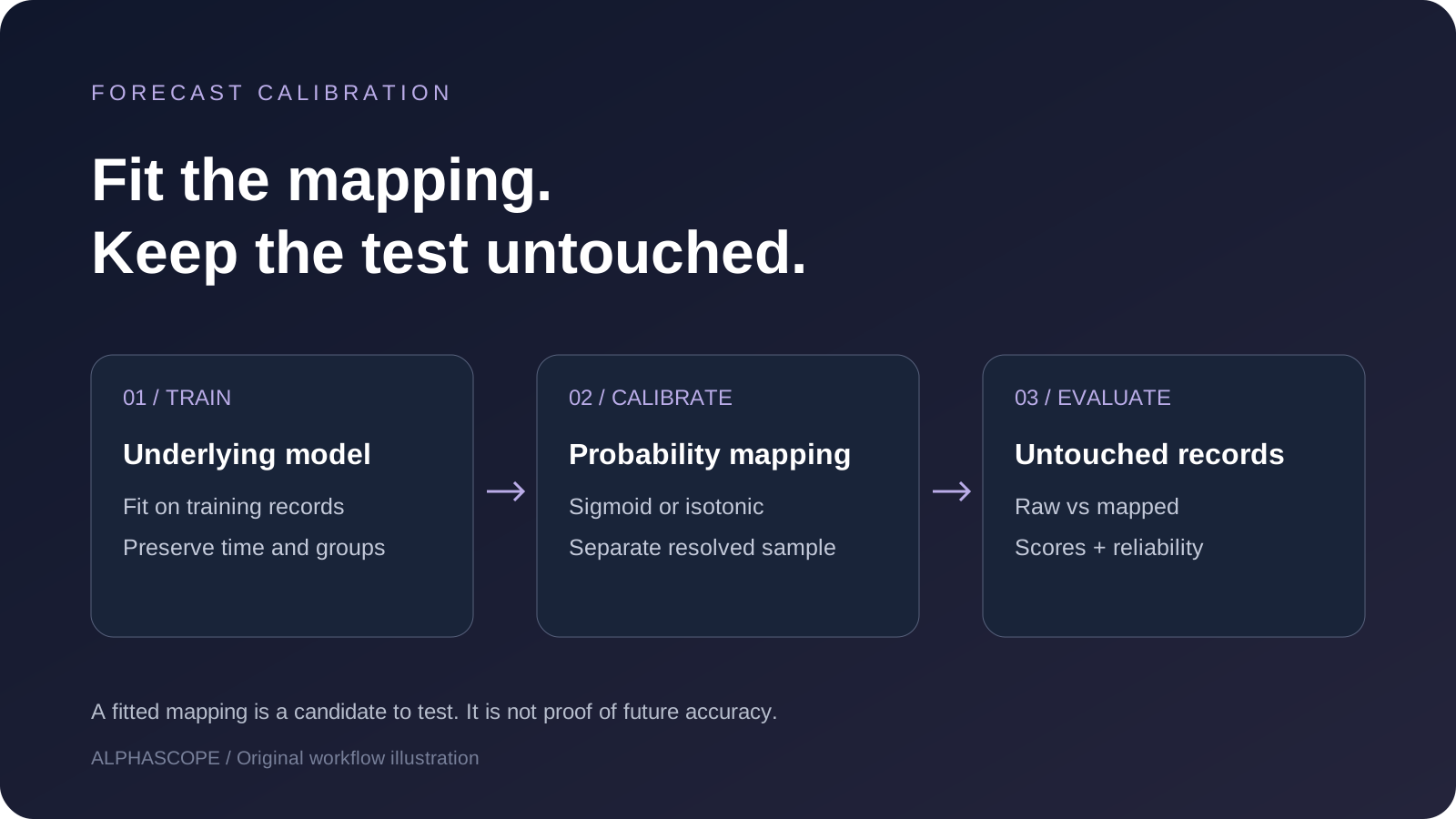
- Training: fit the underlying model using information available at the forecast time.
- Calibration: fit the probability mapping using separate resolved records.
- Evaluation: compare raw and calibrated probabilities on untouched records.
For event forecasts, plan the split around the information timeline. A resolved outcome must be available before you use it to fit a mapping. Keep repeated forecasts for the same event out of competing splits when they would leak information. Fit preprocessing on the permitted training data too. These are design questions that a library class cannot answer for you.
For example, do not train on an early forecast for an election and evaluate on a later forecast for that same election while describing the split as independent. A different timestamp does not create a different outcome. Use event groups and a time boundary appropriate to your intended deployment, and explain any embargo or exclusions.
A runnable CalibratedClassifierCV example
Download the synthetic Python example. It was executed with scikit-learn 1.7.2. Install that version in your own environment with python3 -m pip install scikit-learn==1.7.2, then run python3 forecast-calibration.py. The script prints its installed version.
The example generates 6,000 records and assigns 2,000 each to training, calibration and evaluation. It fits GaussianNB once, wraps that fitted model in FrozenEstimator, then fits separate sigmoid and isotonic calibrators on only the calibration subset. Its evaluated probability column is explicitly the class labelled 1.
The official CalibratedClassifierCV reference explains that FrozenEstimator calibrates an already fitted classifier and leaves the disjoint-data responsibility with you. The class uses decision_function when available, otherwise predict_proba. This example uses a fixed holdout, rather than claiming that default cross-validation validates a time-dependent forecasting process.
calibrated = CalibratedClassifierCV(
    FrozenEstimator(base), method="sigmoid", ensemble=False
).fit(X[calibration], y[calibration])
p = calibrated.predict_proba(X[evaluation])[:, 1]
Both classes occur in the generated subsets, their row indices are disjoint, and returned probabilities are checked for finite values within [0, 1]. The synthetic records are not evidence that your own forecasts satisfy independence, stationarity or data-availability requirements.
What the checked example actually shows
| Version 1.7.2 run | Brier loss | Mean log loss | Evaluation rows |
|---|---|---|---|
| Raw GaussianNB | 0.1247 | 0.4353 | 2,000 |
| Sigmoid | 0.1211 | 0.3948 | 2,000 |
| Isotonic | 0.1192 | 0.4171 | 2,000 |
Lower is better for these two scores. In this run, isotonic has the lowest Brier loss, while sigmoid has the lowest log loss. That disagreement is useful: “best calibrated” needs a stated definition and more evidence than one number. These are generated-data results from one seeded example, not a ranking of the methods for prediction markets.
The script also prints occupied-bin mean probabilities and observed positive frequencies with ten uniform bins. Inspect those pairs and the sample distribution. Our calibration calculator and reliability diagram provides two explicitly labelled interpretations for entered binary records; it does not fit either mapping.
Use the Brier score calculator and log-loss calculator to understand the scoring formulas. Their results describe the entered sample. A forecast metric does not account for executable prices, fees or liquidity and is not a trading-profit estimate.
How temperature scaling differs
Guo and colleagues’ 2017 paper discusses temperature scaling: one positive temperature rescales logits before conversion to probabilities. It is a different parameterization from a sigmoid with an independently fitted slope and intercept. The paper studies classification benchmarks, not Kalshi, Polymarket or Alphascope trading results.
The example in this article runs only sigmoid and isotonic. Do not add a method string without checking your installed library version and its input requirements. The current official API lists temperature support added in version 1.8; the downloadable example is deliberately validated against version 1.7.2.
Before applying a mapping to forecasts
- Save the raw forecast alongside the mapped value and mapping version.
- Define the positive outcome and resolution source before scoring.
- Document data dates, event groups, exclusions and forecast horizons.
- Choose fitting and evaluation rules before comparing results.
- Inspect sparse regions and changes in the events you forecast.
- Retain the original model when the evidence does not support a change.
Sources and example reviewed October 13, 2026. Alphascope helps organize prediction-market research; this guide does not establish that any particular forecasting system is calibrated.