
On this page
A credible interval contains a stated amount of posterior probability for a parameter, conditional on the data, likelihood and prior. A confidence interval has a stated coverage rate as a procedure across repeated samples under its assumptions. The familiar 95% labels do not make those interpretations interchangeable.
Both intervals can concern the same unknown parameter. This differs from the distinction between a parameter interval and a prediction interval for a future observation. The original example below compares intervals for one mean using the same fictional observations and two explicitly stated priors.
Credible interval vs confidence interval
| Question | Bayesian credible interval | Frequentist confidence interval |
|---|---|---|
| What does the level describe? | Posterior probability mass under the specified analysis | Coverage of the interval-generating procedure across repeated samples |
| Does a prior enter the calculation? | Yes, as part of the Bayesian model | No Bayesian prior is needed for the method used here |
| Can the bounds depend on assumptions? | Yes: prior, likelihood and interval definition matter | Yes: sampling model, method and target matter |
| Does 95% guarantee the model is correct? | No | No |
Stan’s posterior-interval documentation explains the data-and-model-conditional probability interpretation and distinguishes it from frequentist confidence. NIST’s confidence-limits explanation describes repeated-sampling coverage: a particular computed interval either contains the fixed parameter or does not.
Original example: same data, different prior information
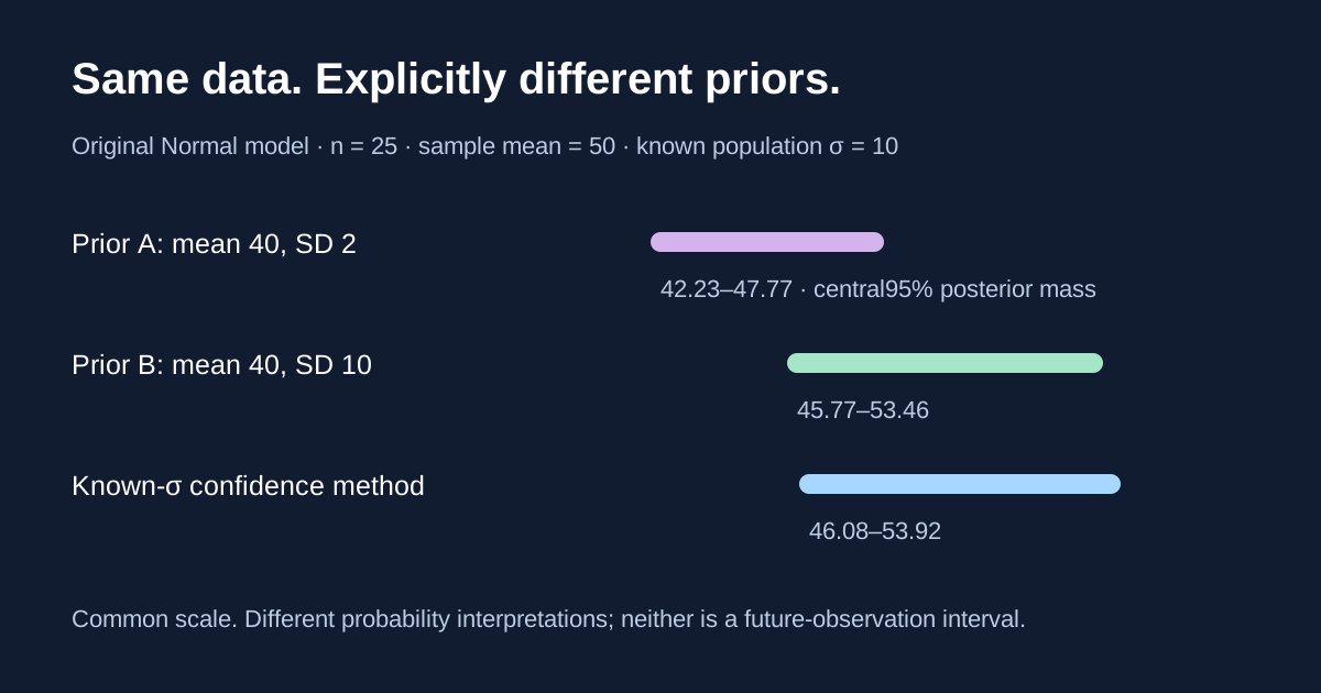
Assume 25 independent observations from a Normal distribution with unknown mean μ and known population standard deviation σ =10 units. Their observed sample mean is 50. These are supplied fictional summaries, not platform results or estimates from a live market.
The sample mean’s variance is σ²/n =100/25 =4, and its standard deviation is 2. Using the standard Normal 97.5th percentile z ≈1.9599639845, the familiar known-σ 95% confidence interval is 50 ±z ×2, or approximately [46.08, 53.92].
This is a known-population-variance construction. NIST also displays a t interval when the variability is estimated; do not substitute an estimated sample standard deviation into this example while silently retaining the same coverage factor.
Calculate a Normal posterior
Now specify a Normal prior for μ with prior mean m₀ and prior variance v₀. The Statistical Proof Book’s Normal known-variance derivation gives a Normal posterior whose precision is the sum of prior and data precision.
For our sample, data precision is n/σ² =25/100 =0.25. Write:
posterior variance v =1 /(1/v₀ +0.25)posterior mean m =v ×(m₀/v₀ +0.25 ×50)central 95% credible interval =m ±z ×sqrt(v)
The last expression applies because the posterior in this stipulated model is Normal. It is not a universal formula for arbitrary posterior shapes.
Two priors, two credible intervals
| Analysis | Prior for μ | Posterior mean | Posterior variance | Rounded central 95% interval |
|---|---|---|---|---|
| Prior A | Normal mean 40, standard deviation 2 | 45 | 2 | [42.23, 47.77] |
| Prior B | Normal mean 40, standard deviation 10 | 49.6154 | 3.8462 | [45.77, 53.46] |
| Known-σ confidence method | No Bayesian prior in this construction | Centered at sample mean 50 | Sample mean variance 4 | [46.08, 53.92] |
For A, prior precision is 1/4 =0.25, equal to data precision. The posterior mean is (0.25 ×40 +0.25 ×50)/0.50 =45, and posterior variance is 2. Its half-width is z ×sqrt(2) ≈2.7718.
For B, prior precision is 1/100 =0.01. Total precision is 0.26, so the posterior variance is 1/0.26 =50/13 and the mean is (0.01 ×40 +0.25 ×50)/0.26 =645/13. Its half-width is approximately 3.8439.
The data have not changed. Prior A exerts a stronger pull toward 40 than B does. Its narrower posterior interval is conditional on that stronger prior; it is not evidence that A is a more accurate description of reality. A prior should be justified before looking for a desired conclusion, and sensitivity to plausible alternatives should be visible.
What can you say about a 95% credible interval?
For Prior A under this model, the posterior assigns 95% probability to μ lying between the unrounded central bounds. That statement conditions on the observed data and the chosen likelihood and prior. It does not mean the likelihood or prior has been verified, or that 95% of future observations lie inside the parameter interval.
Stan defines a central interval using posterior quantiles: for 95%, the endpoints are the 2.5th and 97.5th percentiles. Other credible-interval conventions can produce different endpoints for an asymmetric or multimodal posterior. Name the convention rather than treating every 95% credible set as identical.
For the confidence method, the 95% statement instead concerns the proportion of intervals that would cover a fixed μ in repeated sampling under the model. It is not automatically a posterior-probability statement about the one interval already computed.
A credible interval need not have 95% coverage for every fixed parameter
There is an instructive consequence of Prior A. Under a separate repeated-sampling experiment, hold the true mean fixed at μ =50 and keep σ =10 and n =25. The sample mean then follows a Normal distribution with mean 50 and standard deviation 2.
Prior A’s posterior center is (40 +sample mean)/2, with constant half-width about 2.7718. Its interval contains the fixed value 50 only when the sample mean is approximately between 54.4564 and 65.5436. Under that fixed-μ experiment, the probability of such a sample mean is about 1.29%.
This is an original mathematical illustration of the two different probability questions, not a general empirical indictment of Bayesian methods. Each posterior interval still has its stated posterior mass under Prior A. Fixed-parameter frequentist coverage and posterior mass are different properties. Our confidence construction has 95% repeated-sampling coverage under the stipulated Normal model.
Neither parameter interval is a prediction interval
Both the confidence and credible intervals above target μ. A future individual observation has its own variation in addition to uncertainty about μ. For that distinction, use our prediction interval vs confidence interval guide.
An event forecast such as a 70% probability is also a different object from an interval for a numeric population mean. To review recorded binary probabilities, use the Brier score calculator or log-loss calculator. An interval calculation does not by itself establish profitable trading or accurate market forecasts.
Reproduce the comparison
Download the original Python calculation. It uses the standard library to print posterior parameters, intervals, posterior mass and the fixed-μ coverage illustration. No model is fitted to real observations.
- Name the parameter and distinguish it from any future prediction target.
- Record the sampling model and whether variability is known or estimated.
- For Bayesian analysis, document the prior and its rationale.
- State the interval level and whether it is a central quantile interval.
- Keep posterior probability separate from repeated-sampling coverage.
- Show sensitivity to assumptions before interpreting narrower bounds as better knowledge.
For another explicitly modeled example of uncertain parameters and outcome variation, read epistemic uncertainty. Keep any supporting evidence and forecast updates timestamped when using event research.