
On this page
Epistemic uncertainty concerns what is not known about a model, parameter or explanation. Aleatoric uncertainty concerns outcome variation remaining within a specified model and information set. A useful question is whether more relevant evidence could identify an unknown feature of the process, or whether variation would remain even after that feature was known.
What is epistemic uncertainty?
Hüllermeier and Waegeman’s introduction distinguishes uncertainty associated with missing knowledge from uncertainty associated with random variation. It also emphasizes that inferences depend on model assumptions. Learning can reduce ignorance about a model without making every future outcome certain.
Do not turn this into a universal promise that more data eliminates all epistemic uncertainty or a claim that an observed process is inherently irreducible. The boundary depends on what the model includes and what information is available. A useful label needs a stated object: uncertainty about which parameter, under which assumptions?
Aleatoric vs epistemic uncertainty
| Question | Epistemic aspect | Aleatoric aspect within a model |
|---|---|---|
| What is uncertain? | Which parameter or explanation applies | Which outcome occurs given that parameter |
| What might relevant evidence do? | Help distinguish candidate explanations | Leave residual outcome variation |
| What must be specified? | Candidate models, information and assumptions | The conditional outcome distribution |
| What should not be inferred? | Every uncertainty is removed by a larger dataset | Variation is immutable under every richer model |
Gruber and colleagues’ statistical perspective cautions that uncertainty has multiple sources and does not always admit a simple two-part decomposition. The calculation below is therefore a decomposition for a deliberately specified toy model, not a universal measurement rule.
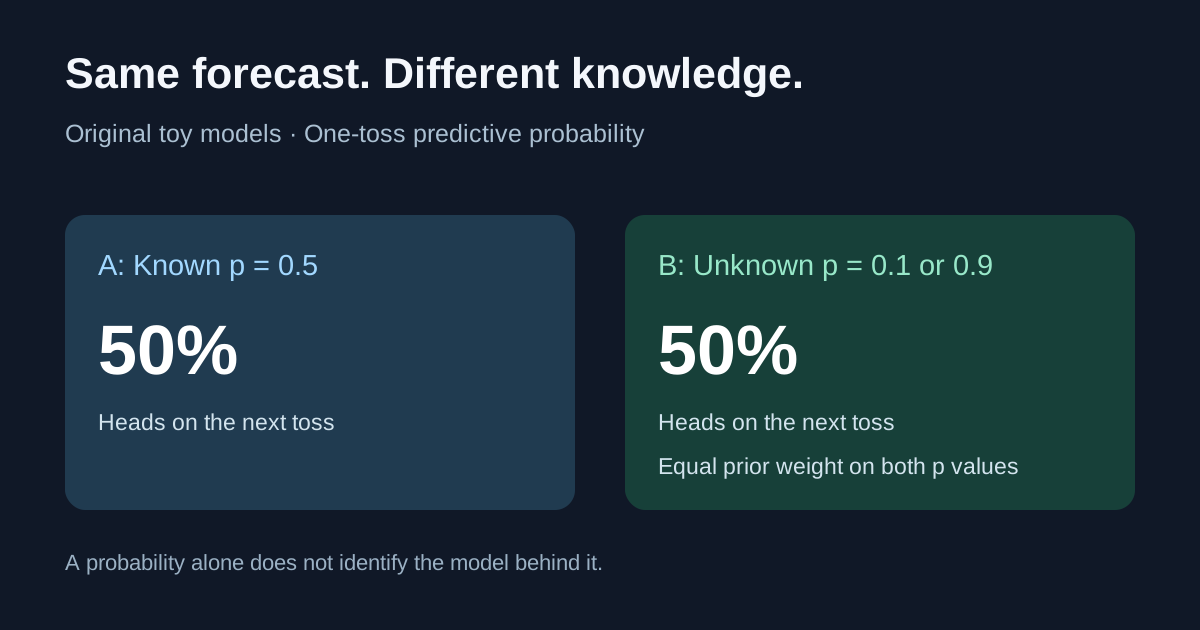
Original example: two models both predict 50% Heads
Consider two different fictional descriptions of coin tossing. Let the next outcome Y equal 1 for Heads and 0 for Tails. These are stipulated probability models, not experiments with physical coins.
- Model A: The Heads probability is known to be p =0.5. Tosses are independent.
- Model B: One coin is selected once and then retained. Its Heads probability is either p =0.1 or p =0.9, each with prior probability 0.5. Tosses are independent conditional on that fixed but unknown p.
Model A assigns 50% to the next Heads directly. Model B assigns 0.5 ×0.1 +0.5 ×0.9 =0.5. Their one-toss predictive distributions are identical. But Model A contains no uncertainty about p, while Model B does.
Keeping the selected coin fixed matters. If a new coin were independently selected for every toss, the learning exercise below would describe a different process.
A worked variance decomposition
For this exercise, use the law of total variance: Var(Y) =E[Var(Y |p)] +Var(E[Y |p]). For a Bernoulli outcome, the conditional mean is p and conditional variance is p ×(1 −p).
| Quantity | Model A: known p =0.5 | Model B: unknown p =0.1 or 0.9 |
|---|---|---|
| Next-toss Heads probability | 0.50 | 0.50 |
| Expected conditional variance | 0.25 | 0.09 |
| Variance of conditional mean | 0 | 0.16 |
| Total predictive variance | 0.25 | 0.25 |
In Model B, either candidate has conditional variance 0.1 ×0.9 =0.09. The two candidate means are each 0.4 away from the overall mean of 0.5, giving 0.5 ×(0.1 −0.5)² +0.5 ×(0.9 −0.5)² =0.16. The pieces sum to 0.25.
Within this assumed model, the 0.09 term represents remaining toss variation conditional on p, and the 0.16 term represents uncertainty over p. Model A puts all 0.25 into conditional variation. These variances are on the numeric 0/1 outcome scale. They are not percentages of confidence or probability points to subtract from the 50% forecast.
What happens after observing one Heads?
Under Model B, a Heads is nine times as likely if p =0.9 as if p =0.1. Bayes’ rule gives:
P(p =0.9 |Heads) =(0.5 ×0.9) /(0.5 ×0.9 +0.5 ×0.1) =0.9.
The next-toss Heads probability becomes 0.9 ×0.9 +0.1 ×0.1 =0.82. The unknown coin has not been identified with certainty. Under Model A, observing a Heads leaves the next independent toss at 0.5 because p was already known.
For Model B after that observation, expected conditional variance remains 0.09. The variance of the conditional mean becomes 0.9 ×(0.9 −0.82)² +0.1 ×(0.1 −0.82)² =0.0576. Their sum is 0.1476, matching 0.82 ×0.18.
This particular observation reduces uncertainty about p under the stipulated setup. It is not a claim that each new observation always reduces every uncertainty measure in every model. Evidence can also reveal a missed explanation or undermine the model itself.
What does this mean for prediction markets?
A displayed 50% Kalshi or Polymarket quote does not tell you whether uncertainty resembles Model A or Model B. The toy calculation proves that even identical one-event probabilities can coexist with different assumed uncertainty over a parameter. It does not show that a trading price encodes either decomposition.
For an actual question, distinguish the defined outcome, your evidence, your model and the quote being observed. Save the exact contract, time, bid or ask, and available size. Then ask what missing evidence could change your probability and what variation would remain under your stated model.
A wider range of analyst estimates is not automatically a quantified epistemic-uncertainty measure. The analysts may use different event definitions, share sources or omit the same explanation. Our wisdom-of-crowds guide discusses participation and shared errors.
For the separate question of preferences toward unclear probabilities, see ambiguity aversion and the paired-choice example.
When comparing market activity, keep forecast uncertainty separate from volume and open interest: neither count alone measures forecast quality.
A practical uncertainty worksheet
- Define the target. Specify the event, deadline and resolution source.
- Name the model. State candidate explanations, unknown parameters and assumptions.
- List missing information. Identify an observation that could distinguish those explanations.
- State the residual. Explain what remains uncertain even if that observation arrives.
- Check model limits. Ask whether the candidate set excludes a plausible explanation.
- Save and review. Record the forecast before resolution and explain later changes.
If you have only a probability and no supporting model, do not invent a numeric split between epistemic and aleatoric uncertainty. State what is known and what remains unmeasured. For evaluating saved confidence claims, see overconfidence bias examples.
Alphascope’s market news can support source gathering. A new headline is useful when it changes the evidence for a defined question; more headlines alone do not establish that uncertainty has been measured or reduced.