
On this page
Forecast error is the observed value minus the forecast made for that value. With the convention error =actual −forecast, a positive error means the actual exceeded the forecast; a negative error means the forecast was too high. State the sign convention because some workflows reverse it.
One error describes one prediction. A summary such as mean error, mean absolute error or root mean squared error answers a different question about a set of predictions. The worked dataset below is original and fictional; it does not measure Alphascope or any forecasting platform’s performance.
Forecast error formula
For a forecast issued at time T for an observation h steps later, write e(T+h) =y(T+h) −forecast(T+h |T). The notation after the vertical bar records what information date the forecast used. The horizon h matters: a forecast made a month ahead is a different evaluation task from an update made an hour ahead.
Forecasting: Principles and Practice distinguishes test-set forecast errors from training residuals. Its evaluation chapter emphasizes forecasts assessed on new observations rather than judging future performance solely by the fit to training data.
Original calculation: mean error zero, forecasts still miss
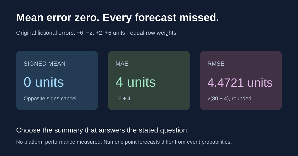
Suppose a fictional analyst records four forecasts of 20 units, each before its target is observed and at the same predefined horizon. The four later observations are 14, 18, 22 and 26 units. Treat every row as equally weighted.
| Case | Actual | Forecast | Error: actual −forecast | Absolute error | Squared error |
|---|---|---|---|---|---|
| A | 14 | 20 | −6 | 6 | 36 |
| B | 18 | 20 | −2 | 2 | 4 |
| C | 22 | 20 | 2 | 2 | 4 |
| D | 26 | 20 | 6 | 6 | 36 |
| Total | 80 | 80 | 0 | 16 | 80 |
The signed mean error is (−6 −2 +2 +6) ÷4 =0. This describes cancellation between overforecasts and underforecasts in this sample. It does not mean every forecast was correct: none was.
The forecast total and actual total both equal 80, so aggregate total error is also zero. A workflow that only checks the total would miss the row-level discrepancies. Whether those discrepancies matter operationally depends on the decision being supported.
Mean error vs MAE vs RMSE
Hyndman and Koehler’s author-hosted paper on forecast-accuracy measures defines the common absolute- and squared-error summaries. Apply each formula to the same eligible observations.
| Measure | Formula | Our fictional result | Interpretation |
|---|---|---|---|
| Mean error | mean(error) | 0 units | Signed average; opposite errors can cancel |
| MAE | mean(abs(error)) | 16 ÷4 =4 units | Average absolute miss |
| MSE | mean(error²) | 80 ÷4 =20 squared units | Average squared miss |
| RMSE | sqrt(mean(error²)) | sqrt(20) ≈4.4721 units | Root of the average squared miss |
RMSE is not the mean error, and it is not the square root of MAE. For these rows, taking the square root of 4 would produce 2, which is not the RMSE. Keep the sequence explicit: square each signed error, average the squares, then take the square root.
MAE and RMSE retain the target’s units; MSE has squared units. Neither “4 units MAE” nor “4.4721 units RMSE” is automatically an accuracy percentage.
Two forecasts can have the same MAE and different RMSE
As a separate candidate on exactly the same four targets, suppose an alternative had forecast 22 for each case. Its errors are −8, −4, 0 and 4. Their absolute values still sum to 16, so its MAE is also 4.
Its squared errors sum to 64 +16 +0 +16 =96, producing RMSE =sqrt(96 ÷4) =sqrt(24) ≈4.8990. Compared with the original, it has equal MAE and higher RMSE in this constructed sample.
The difference comes from how the misses are distributed. It does not prove which forecasting method will work better next time or that one metric is always the right decision criterion. Predefine the loss that matches the use case, and retain the individual errors rather than only the winning summary.
Percentage forecast error and the zero problem
For an actual value with a meaningful nonzero denominator, signed percentage error is 100 ×(actual −forecast) ÷actual. MAPE averages the absolute percentage errors. The Hyndman–Koehler paper discusses undefined values at zero, unstable behavior near zero, and the need for a meaningful zero point.
In a separate invented case, an actual of 10 and forecast of 12 gives −2 units and −20% signed error. Its absolute percentage error is 20%. This is one row’s error, not a general claim that the model is “80% accurate.”
If the actual is zero and the forecast is 2, the unit error is −2 but the percentage expression divides by zero. Do not quietly delete that row, replace it with zero percentage error or report a normal MAPE without documenting a defensible treatment. Changing the denominator creates a different metric that needs its own name and definition.
Forecast error vs residual
A fitted residual compares an observation used in estimation with a corresponding fitted value. A held-out forecast error evaluates a prediction for an observation outside that fitting sample. The textbook’s distinction also notes that forecast errors may concern multiple steps ahead.
As an original evaluation design, imagine fitting through December and recording January, February and March forecasts at that December cutoff. Those forecasts have horizons one, two and three months. An updated March forecast issued after February data becomes available has a different information cutoff; label it separately instead of silently substituting it for the December-issued forecast.
Keep model selection and final assessment separate. If you repeatedly choose a model using the same evaluation rows, those rows have influenced the choice. Preserve a later assessment period or another defensible evaluation design. A tiny illustrative sample like ours cannot establish stable real-world performance.
For event probabilities, use a probability score
A numeric point forecast and an event probability are different prediction objects. “The count will be 20” is a point forecast. “The event has a 70% chance” assigns probability to a defined outcome. Do not score a probability as if it were a forecast of a count in units.
The official scoringrules Brier-score reference gives the binary squared-probability-error convention. For an original example, a recorded probability p =0.70 and outcome y =0 gives (0.70 −0)² =0.49. A single realized outcome is not a calibration study.
Use our existing Brier score calculator and log-loss calculator for probability scoring. Our Polymarket accuracy guide explains why a defined sample, forecast horizon and resolution rules matter when evaluating event-market probabilities.
For numeric uncertainty ranges rather than single point predictions, compare prediction intervals and confidence intervals. They answer different questions about future observations and population parameters.
A forecast-error review worksheet
- Define the target, its units and the observed outcome source.
- Record the forecast value, issue date, target date and horizon.
- State the sign convention and preserve each row’s error.
- Separate training residuals from held-out forecast errors.
- Choose signed, absolute, squared or probabilistic summaries for the stated task.
- Report missing values, zero denominators, exclusions and weighting.
- Compare methods on the same targets and information cutoffs.
Download the original worked ledger and blank review fields. For constructing a forecast from comparable past cases before evaluating it, read reference class forecasting. Keep evidence gathered through event research timestamped so later information does not leak into an earlier forecast record.