
On this page
Look-ahead bias occurs when a historical decision uses information that would not have been available when that decision was made. The result may look like forecasting skill while actually benefiting from future knowledge.
The test is not simply whether a row’s date precedes a trade. Ask when its exact version was published, when the system received it, and when the model could use it. A historical observation can acquire a future revision.
What is look-ahead bias?
QuantConnect’s research documentation defines the problem in terms of information unavailable at decision time. It gives examples involving closing-price decisions filled at that same close, training on future data and selecting a universe using later performance.
This page develops an original point-in-time feature example and a downloadable offline check. It is not a backtest of Alphascope, Kalshi, Polymarket or an actual trading strategy.
Observation time is not availability time
| Clock | What it records | Why it matters |
|---|---|---|
| Observed period | When the measured event or period occurred | The value may be published later |
| Publication time | When the exact version became public | A revision has its own release time |
| Ingestion time | When the research or trading system received it | A public release may still be unavailable to that system |
| Feature-ready time | When transformations finish | Processing can introduce another delay |
| Decision time | When the forecast or order decision is frozen | Defines the information cutoff |
A realistic availability rule accounts for every relevant delay. In the deliberately small fixture below, publication and ingestion are recorded explicitly and there is no additional processing delay. The effective availability is their maximum.
Original example: a future revision enters an earlier decision
Construct three fictional versions of one synthetic feature. These are not economic observations or actual model forecasts. All times below are UTC.
| Version | Observed period | Published | Ingested | Feature value |
|---|---|---|---|---|
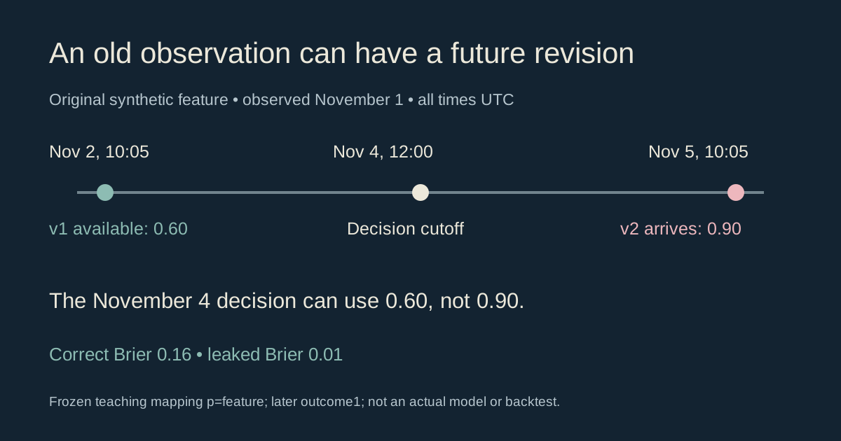
| v1 | November 1 | November 2, 10:00 | November 2, 10:05 | 0.60 |
| v2, revision of the same period | November 1 | November 5, 10:00 | November 5, 10:05 | 0.90 |
| Next observed period | November 4 | November 6, 10:00 | November 6, 10:05 | 0.70 |
Freeze a historical decision at November 4, 12:00 UTC. Only v1 is available. The revision refers to November 1 but arrives on November 5. The next observation refers to November 4 but is not published until November 6.
A later download that replaces November 1’s original value with its final revision would supply 0.90 to the November 4 decision. Filtering only on the observation date would not catch the mistake. It is the wrong vintage for the decision’s information set.
How leakage can improve a forecast score without improving a model
For this original teaching calculation only, freeze the mapping forecast probability =feature value. Stipulate that the binary outcome, evaluated later, is 1. There is no fitted model, live price or financial return in this example.
The correctly timed forecast is 0.60. Its binary Brier score is (0.60 −1)² =0.16. Substituting the unavailable revision gives (0.90 −1)² =0.01.
The apparent score improvement is 0.15, produced entirely by changing which information the historical decision can see. It does not establish forecasting skill. One constructed observation also cannot establish calibration or a statistically meaningful performance difference.
Use the Brier score calculator for scoring a defined forecast record. A scoring formula can be correct even when its historical input probabilities are contaminated.
A point-in-time join needs the correct version
For the fixture, first retain records whose observed period and effective availability are both no later than the decision. Then select the latest eligible observed period and its latest eligible version.
eligible =observed_at ≤decision_at AND available_at ≤decision_at
That is more restrictive than an ordinary date merge. Joining to the nearest timestamp can select a future observation if forward matches are allowed. Sorting the final revised dataset chronologically does not recover the version history it discarded.
The example treats equal-time availability as inclusive and assumes the record is fully usable at that timestamp. In a live system, arrival ordering, clock precision and processing can make a strict cutoff or an explicit buffer necessary. Document the decision rule rather than inferring availability from equal-looking rounded timestamps.
Publication and ingestion delays both matter
Move the fictional decision to November 5 at 10:02. The revision has been published but is not ingested until 10:05, so the system still uses v1. At 10:05, under the fixture’s inclusive rule, v2 becomes eligible.
If an archive proves only publication time, it does not independently prove when your historical system received the record. Conversely, today’s ingestion timestamp cannot reconstruct the old receipt time. Preserve source and system clocks separately.
QuantConnect’s reconciliation guide notes that custom data can still introduce look-ahead bias and that data should be emitted after its relevant period. A platform’s time controls do not automatically validate every external dataset.
Economic-data revisions and ALFRED vintages
The St. Louis Fed’s real-time period documentation distinguishes information known today about the past from information known in a past period. It explains that observation values can be revised and that real-time periods can retrieve historical vintages.
A vintage can be useful evidence about which version existed, but a date-level vintage alone does not establish exact intraday publication or your system’s receipt time. A noon decision may require finer timing than a date-only record supplies.
Do not automatically replace every historical feature with the latest corrected value. Preserve revisions as separate versions and decide which version was usable at each forecast cutoff. Our numerical fixture is synthetic and is not a claim about any actual FRED series.
Look-ahead bias in machine learning and preprocessing
scikit-learn’s data-leakage guidance explains that test data should not determine fitted preprocessing or model choices. It recommends separating training/test data before learning transformations and using pipelines to keep fitting in the appropriate subset.
For time-ordered forecasting, feature versions, labels, preprocessing and model-training time all need cutoffs. A scaler fitted on the full historical-plus-future sample can leak information even when the final prediction function receives only past-dated rows.
A chronological split is necessary in many forecasting designs but is not a complete proof. A training row’s label might become known after the model’s supposed training cutoff, or overlapping events may share information across the split. Check availability of labels as well as features.
Prediction-market examples: prices, news and resolution labels
- Final outcome as a feature: A later resolution label can be used for evaluation, but not as information available to the earlier forecast.
- Updated market rules: Today’s description may include clarification posted after a historical decision.
- News edits: A story’s original publication date does not prove that its current text was present in the first version.
- Closing prices: A price used to generate a signal may not also be an executable fill after that signal is computed.
- Selected markets: Choosing only markets still discoverable today can omit relevant historical cases.
These are constructed failure modes to investigate, not claims that a particular venue’s current dataset is defective. For platform data, save exact market identity, quote time, collection time and source version rather than only a title and outcome.
Look-ahead bias vs survivorship bias and overfitting
Look-ahead bias concerns the information set at decision time. Survivorship bias concerns which cases remain in the sample. Overfitting concerns adapting choices to noise or repeatedly selected historical results.
The problems can overlap, but correcting one does not prove the others are absent. For example, preserving old feature vintages does not restore markets missing from the research universe. Likewise, a separate final test set loses its role if its outcomes repeatedly guide changes.
Reproduce the point-in-time example in Python
Download the original offline availability-time example. Run python3 look-ahead-bias.py. It uses standard-library timezone-aware datetimes and Decimal arithmetic, with no data feeds, credentials or orders.
The fixture checks the initial decision, an ingested-late revision, the next observed period, a missing early observation, row-order independence and duplicate-version rejection. It reproduces Brier scores 0.16 and 0.01 using the supplied identity mapping and later outcome.
The script tests one feature-selection rule. It does not implement model training, time-series cross-validation, order execution or a full leakage audit. Passing it does not validate an actual trading backtest.
For a separate evaluation schedule, see our walk-forward analysis guide. It provides expanding/rolling windows, label-availability checks and a complete out-of-sample scoring fixture.
A look-ahead bias audit checklist
- Freeze the decision time, forecast and model version.
- Preserve observation, publication, ingestion and feature-ready times.
- Keep revisions instead of overwriting historical values.
- Join only to eligible versions under a stated availability rule.
- Check when training labels became known.
- Fit transformations within the appropriate training subset.
- Separate signal creation from realistic execution assumptions.
- Keep outcome evaluation downstream of the frozen forecast.
- Record missing data and universe changes explicitly.
Our prediction-market backtesting guide covers the broader workflow. Alphascope’s market-linked research provides event context; research quality still depends on showing what was knowable at the time.