
On this page
Walk-forward analysis evaluates a forecasting procedure by repeatedly fitting on eligible earlier data and testing on a later block. The cutoff moves forward, the procedure is refitted under predeclared rules, and each test forecast is evaluated after its outcome becomes known.
It is a way to examine out-of-sample behavior over time, not a guarantee of trading profitability or freedom from leakage. The data versions, label availability, fitting rules and execution assumptions still matter.
What is walk-forward analysis?
Forecasting: Principles and Practice describes time-series cross-validation using earlier training observations and later test observations, with the forecasting origin moving forward. It also discusses evaluating more than one forecast horizon.
The crucial separation is between fitting a procedure and observing how its frozen predictions perform later. Re-estimating a model at the next scheduled origin can be part of the procedure; changing the procedure after inspecting a test failure is a research decision that needs separate evaluation.
Expanding vs rolling training windows
| Design | What happens to training history | Tradeoff to investigate |
|---|---|---|
| Expanding window | Keeps eligible earlier observations and adds newly eligible ones | More history, potentially including older relationships |
| Rolling window | Keeps a bounded recent training window | More recent information, fewer retained observations |
| Single holdout | Uses one later evaluation block | Simpler design, fewer distinct evaluation periods |
Neither expanding nor rolling is universally superior. Choosing the window after viewing all its test results can create another selection problem. Record the window rule and selection process with the result.
Original walk-forward schedule
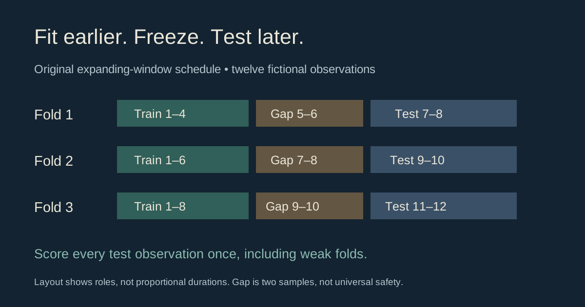
Construct twelve equally spaced fictional forecast observations, numbered 1 through 12. Use four initial training observations, a two-observation gap and two-observation test blocks. The expanding schedule is:
| Fold | Training candidates | Excluded gap | Test block |
|---|---|---|---|
| 1 | 1–4 | 5–6 | 7–8 |
| 2 | 1–6 | 7–8 | 9–10 |
| 3 | 1–8 | 9–10 | 11–12 |
A four-observation rolling cap would instead retain training candidates 1–4, then 3–6, then 5–8. The test blocks remain 7–8, 9–10 and 11–12. These are supplied teaching choices, not recommended sample sizes for an actual model.
Previous test observations may enter a later training window once they are eligible and their labels are known. That is not inherently leakage: the later model has a later cutoff. Their earlier predictions must remain frozen in the evaluation record.
A gap is not a substitute for label-availability checks
In this original fixture, observation i is forecast on synthetic day i and its label arrives on day i +2. Fit each model just before its first test day, requiring training labels to have arrived strictly before that time.
For fold 1, labels for observations 1–4 have arrived by days 3–6, before test day 7. Observation 5’s label arrives on day 7 and does not meet the strict cutoff. The gap therefore has an explicit role in this fixture.
In a real event dataset, some labels might resolve much later than others. Two omitted rows do not necessarily represent two days, let alone a safe information boundary. Apply each row’s actual availability and any relevant overlap or grouping rules.
The scikit-learn TimeSeriesSplit reference defines gap as a number of excluded samples and documents test_size and max_train_size. It notes that equally spaced samples are needed for folds covering comparable durations. A splitter cannot infer a prediction market’s resolution time from its row number.
Freeze a simple training rule before scoring
Supply the fictional binary outcomes:
1, 0, 1, 0, 1, 1, 0, 1, 0, 0, 1, 1
Use one predeclared estimator: probability =(training successes +1) /(training observations +2). This is a smoothed frequency rule for illustration, not a tuned trading model or a recommendation to assume all events have the same probability.
Fold 1 has two successes among four training observations, giving 3/6 =0.50. Fold 2 has four among six, giving 5/8 =0.625. Fold 3 has five among eight, giving 6/10 =0.60.
Freeze each probability for its two-observation test block. There is no within-block refitting. Scoring happens later, after the test labels are available; the labels are not consulted while producing those forecasts.
Report all out-of-sample results
| Fold | Frozen probability | Later test outcomes | Mean binary Brier score |
|---|---|---|---|
| 1 | 0.50 | 0, 1 | 0.250000 |
| 2 | 0.625 | 0, 0 | 0.390625 |
| 3 | 0.60 | 1, 1 | 0.160000 |
Across six unique test forecasts, pooled Brier score is 0.266875. A fixed 0.50 baseline scores 0.250000 on those same observations. Lower is better for this score, so the illustrative estimator is worse by 0.016875.
Reporting only fold 3’s 0.16 would hide the weaker periods. This tiny constructed sample cannot support a statistical claim of superiority, infer calibration or establish an economic edge. It simply makes the complete scoring ledger visible.
Here every fold has two tests, so averaging fold means equals pooling individual losses. With unequal test counts, an unweighted average of fold means answers a different question. State the aggregation unit and weights.
Our Brier score calculator explains scoring a defined binary forecast record. A forecasting score is separate from a trade’s fees, payout, slippage and realized return.
Walk-forward validation vs walk-forward optimization
Validation evaluates a specified procedure. Optimization adds choices, such as selecting a threshold, model setting or window length. If choices are made, keep their search within data eligible before the outer test block.
For example, a fictional researcher might compare candidate settings using earlier inner training/validation periods, select one, then freeze it for the next outer block. The outer test is for evaluation, not another tuning target. Our small example does not perform that search.
If you use the three outer results to choose among many redesigned procedures, treat them as development evidence. A separately protected later evaluation can help assess the chosen procedure, but repeatedly inspecting and adapting to that later set also changes its role.
Walk-forward analysis in Python
Download the original offline walk-forward fixture. Run python3 walk-forward-analysis.py. It uses standard-library Fraction arithmetic, so the published scores are checked exactly rather than through rounded intermediate values.
The script constructs expanding and rolling windows, checks delayed training labels, freezes block forecasts before scoring, and verifies unique test observations and invalid-window rejection. It reproduces the three probabilities and all fold/baseline scores.
It has no dependency on scikit-learn and does not claim to reproduce that library’s complete API. It also does not implement a production model, nested parameter search, live execution, event-group purging or a full point-in-time dataset.
Using the design in prediction-market research
- Separate events from rows. Multiple prices or outcomes for the same underlying event can share information.
- Respect resolution delays. A historical forecast may be old enough to look eligible while its label was still unknown.
- Freeze feature versions. Later news edits, rule changes and revised data must not silently enter older decisions.
- Define the horizon. A price forecast, event-outcome probability and simulated holding-period return are different targets.
- Match evaluation scope. Keep market identity, venue, units, exclusions and timestamps beside the results.
The look-ahead bias guide demonstrates observation versus availability time with another original fixture. A chronological window schedule is useful structure, but the actual information set still needs evidence.
A reproducible walk-forward analysis checklist
- Specify the forecast target, horizon and research universe.
- Choose expanding or rolling windows and the refit schedule.
- Define feature and label availability cutoffs.
- Declare gap, overlap and event-group handling rules.
- Keep any parameter selection inside eligible earlier data.
- Store frozen predictions before evaluating outcomes.
- Score every eligible test case against a stated baseline.
- Report missing cases, exclusions, fold sizes and pooled results.
- Separate forecast quality from simulated execution and actual returns.
Our prediction-market backtesting guide covers the broader workflow. Alphascope’s market-linked research adds event context; an evaluation design must still show what was known, fitted and tested at each origin.