
On this page
LMSR stands for logarithmic market scoring rule. In prediction markets, it can define an automated market maker whose prices change as outcome-share quantities change. A trade is priced by the change in a cost function, rather than by multiplying its size by the first displayed marginal price.
This guide uses the standard fixed-liquidity, fee-free mathematical model. It is not a live exchange, a funded market maker or a claim that a particular venue uses LMSR. The primary references are Robin Hanson’s market-scoring-rule paper and Chen and Wortman Vaughan’s cost-function overview, reviewed November 21, 2026.
What the LMSR formula means
Assume n mutually exclusive, collectively exhaustive outcomes and a unit payoff to each share of the winning outcome. Let qᵢ be the net quantity of outcome i shares held by traders in the model. The fixed parameter b is positive and controls the price response.
C(q) = b × ln(Σᵢ exp(qᵢ / b))
pᵢ(q) = exp(qᵢ / b) / Σⱼ exp(qⱼ / b)
Trade payment = C(q + Δq) − C(q)
Here ln is the natural logarithm, and pᵢ is the instantaneous marginal price. The prices sum to one. That algebraic normalization does not prove that the resulting prices match real-world probabilities or that traders have accurate information.
The cost function has an additive starting value. At a zero inventory state with n outcomes, C(0) = b ln(n). For a new trade, subtract the starting cost: charging C(q + Δq) by itself would incorrectly include that initial constant.
LMSR pricing example: buying ten Yes shares
Take a fictional binary market starting at q = (0, 0), with b = 10. Its Yes and No marginal prices are each 0.50. Buy ten Yes shares, moving the inventory to (10, 0):
Starting cost: 10 × ln(2) ≈ 6.931472
Ending cost: 10 × ln(exp(1) + 1) ≈ 13.132617
Payment: 13.132617 − 6.931472 ≈ 6.201145
Average purchase price: 6.201145 / 10 ≈ 0.620115
Ending Yes marginal price: exp(1)/(exp(1) + 1) ≈ 0.731059
The initial price, average paid and final marginal price answer different questions. Multiplying ten by the initial 0.50 gives 5.00 and understates the model’s payment by about 1.201145. Multiplying by the final 0.731059 instead overstates it. The cost difference integrates the changing price along the trade.
If Yes wins, these ten shares pay ten units, producing a trader gain of about 3.798855 before any other costs. If No wins, they pay zero and the trader loses the entire 6.201145 purchase cost. There is no guaranteed return.
The liquidity parameter b: smoother prices require a larger subsidy bound
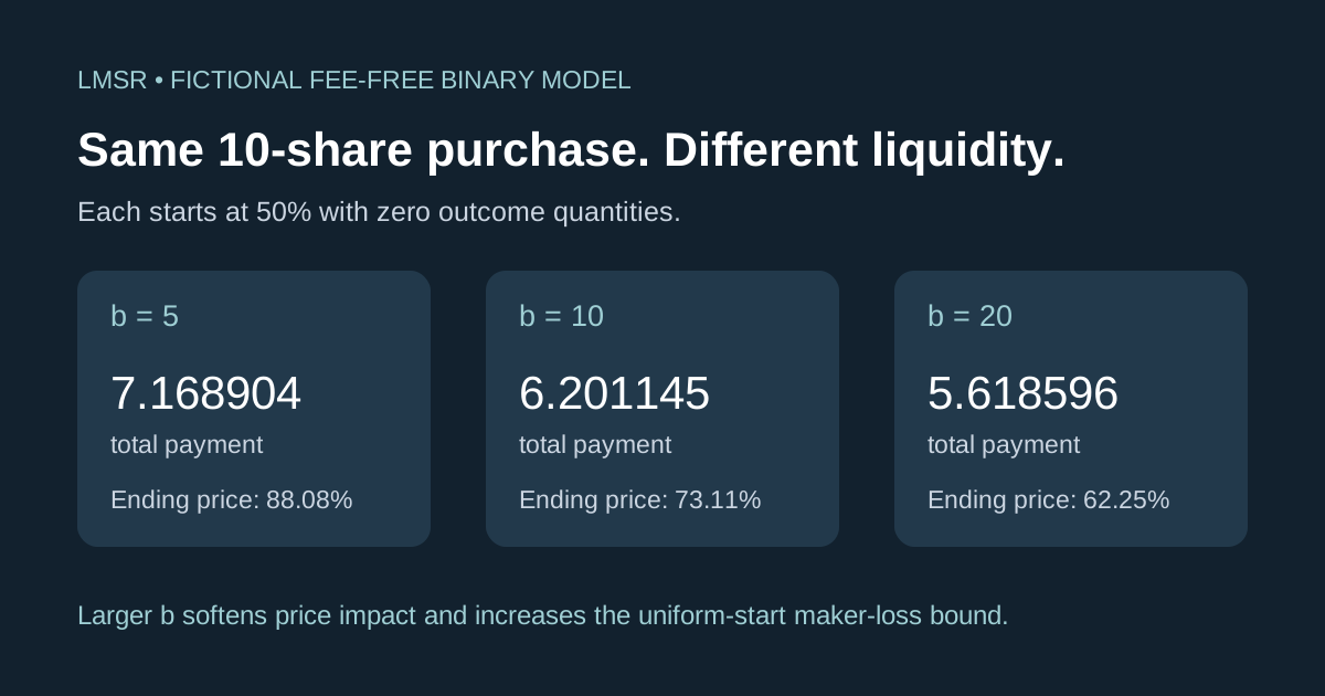
Keep the same zero starting inventory and the same ten-share Yes purchase. Change only b:
| b | Trade payment | Ending Yes marginal price | Uniform-start binary maker-loss bound |
|---|---|---|---|
| 5 | 7.168904 | 88.0797% | 3.465736 |
| 10 | 6.201145 | 73.1059% | 6.931472 |
| 20 | 5.618596 | 62.2459% | 13.862944 |
A larger b makes this fixed-size trade move the price less. In the same standard model, it also raises the organizer’s worst-case loss bound. It is therefore a design trade-off, not a free improvement in liquidity. The numbers are units of the hypothetical market’s payoff currency, not a current exchange fee quote.
The binary marginal-price slope is p(1 − p)/b with respect to its own outcome quantity while the other quantity stays fixed. At a 50% starting price, that slope is 1/(4b). It describes a local change, not the average price for a finite trade.
Why the market maker’s loss is bounded by b ln(n)
Use the zero starting state, fixed b, the complete n-outcome event and no fees or external transfers. If the final inventory is q, the maker has collected C(q) − C(0). If outcome i wins, the model’s payout liability is qᵢ. Thus:
Maker loss if i wins = qᵢ − [C(q) − C(0)]
Since C(q) ≥ maxⱼ qⱼ ≥ qᵢ:
Maker loss ≤ C(0) = b ln(n)
This is a bound for the organizer under these assumptions. It does not say that every trader’s loss is limited to b ln(n). With b = 10, a hypothetical purchase of 100 Yes shares from the zero state costs about 93.068982. The buyer can lose that full amount if No wins, even though the uniform-start binary maker bound is only about 6.931472.
The bound can be approached as one outcome’s quantity becomes very large. It is not a per-trade fee, a promised organizer profit or a proof that a funded implementation is solvent. Resolution, custody, software, transfers and a changed pricing rule require separate accounting.
Initialization matters. If a model starts at a nonzero virtual state q⁰ with prices p⁰, and liabilities are measured as quantity changes from that state, the corresponding outcome-i bound is C(q⁰) − q⁰ᵢ = −b ln(p⁰ᵢ). The worst bound is the largest of those values. A 90%/10% start with b = 10 therefore has an approximately 23.025851 worst-outcome bound under that convention, rather than the uniform 6.931472 bound. State the initial liabilities and cash convention before using either result.
Splitting trades does not remove the model’s price impact
In the unchanged, fee-free cost-function model, buying four shares and then six shares has the same total payment as buying ten at once:
[C(4, 0) − C(0, 0)] + [C(10, 0) − C(4, 0)]
= C(10, 0) − C(0, 0)
The middle costs cancel. This requires the same path endpoints and no intervening trades or rule changes. Per-transaction fees, rounding or other participants changing the inventory can alter a real implementation’s result. Similarly, reversing a trade immediately at the same unchanged fee-free rule reverses its cost; that is not a promise of a free round trip on a live venue.
LMSR vs an order book
| Question | Standard LMSR model | Order-book interpretation |
|---|---|---|
| Where does the next price come from? | A cost-function derivative | Available compatible orders |
| How is a finite trade priced? | A difference of costs | Actual fills across price levels |
| What supplies trading capacity? | The mechanism and its funding assumptions | Resting or newly submitted counterparty orders |
| What does a displayed price establish? | A marginal model price | A field such as bid, ask, midpoint or last trade |
Polymarket’s current international documentation describes a central limit order book, with matching and settlement distinct. Do not use this LMSR worksheet as a Polymarket quote engine. A negative-risk position conversion also does not, by itself, establish LMSR pricing; see our separate negative-risk guide.
For order-book examples, use the slippage calculator with supplied levels and quantities. The broader market microstructure guide explains why a displayed probability and a full-size execution price can differ.
Python example and numerical checks
The standard-library LMSR worksheet reproduces the ten-share examples, ending prices and maker bounds. It uses a centered log-sum-exp calculation to avoid directly exponentiating very large positive inventory values. It also checks split-trade telescoping, reversed trades, uniform quantity shifts, probability sums and the bound over a finite inventory grid.
The worksheet is educational floating-point arithmetic, not production market-maker software. Extreme scales can still lose precision; the finite grid is a check, not the general proof above. It does not manage collateral, authenticate users, enforce real position limits, price external fees or submit orders.
Finally, distinguish LMSR from log loss for forecast evaluation. They share a logarithmic scoring background, but one describes a trading mechanism and the other scores recorded probabilities against outcomes. Neither a smooth price curve nor a good forecast score establishes profitable trading. Explore Alphascope for prediction-market research and compare the exact market rules before applying a model.